

Bioenergetics · OSF-BIO-088
Two-level bioenergetic coherence model: NAD+, ROS and ATP in the ISHEA Δ±1 framework
By Carlos J. Pérez Pulido · ISHEA Institute ·
A theoretical model reading cellular metabolism as two layers: NAD+ redox balance and ROS signalling as regulation, ATP as execution, scored on a bounded coherence metric from −1 to +1
Preprint — Manuscript deposited on OSF. Not peer-reviewed.
Aquí tienes una descripción breve, estilo Wikipedia (neutral y enciclopédica):
The ISHEA Δ±1 Two-Level Bioenergetic Coherence Model is a theoretical mathematical framework that conceptualizes cellular metabolism as a two-layered system integrating redox regulation and energy execution. The model proposes that NAD⁺-dependent redox balance and regulated reactive oxygen species (ROS) signaling form an upstream informational-regulatory layer, while adenosine triphosphate (ATP) functions as a downstream energetic execution layer.
Within the ISHEA Δ±1 framework, systemic bioenergetic states are represented using a bounded nonlinear coherence metric ranging from −1 to +1. The model incorporates weighted contributions and interaction terms between normalized biological variables and uses computational sensitivity analyses to evaluate parameter influence.
It is presented as a systems biology approach to modeling bioenergetic organization and does not constitute a clinically validated diagnostic tool.
Supplementary Material: Energy and Proteic Periodic Tables
- Energy Periodic Table
Purpose:
Organizes and visualizes the energy components of biological and physical systems according to their coherence potential, functional role, and interactions with other elements.
Axes:
X-axis (Energy type):
Metabolic, electrical, mechanical, thermal, informational.
Y-axis (Coherence capacity):
Low → Medium → High. Represents the potential to generate organized information flow efficiently.
Cells:
Each cell represents an “energy element,” for example:
Element Energy Type Function Notes
ATP Metabolic Direct cellular energy High coherence potential; central to metabolism and signaling
FOXP Regulatory protein Neuro-energetic and genetic modulation Influences stress control and neural organization
Cortisol Hormonal Metabolism and stress regulation Excess levels reduce coherence
Δ±1 Index Informational / Physical Integrated planetary energy state measurement Correlates energy flows with dynamic systems
Glucose Metabolic Primary energy source Needs conversion for maximal coherence
Interpretation:
This table helps identify which energies are synergistic vs. which may induce dispersion or incoherence, from cellular to global scales.
- Proteic Periodic Table
Purpose:
Organizes amino acids and peptides according to bioenergetic coherence potential, molecular functionality, and self-organization capacity.
Axes:
X-axis (Amino acids / Peptides):
From simple monomers (glycine, alanine) to peptides formed under non-equilibrium conditions (dipeptides, tripeptides, etc.).
Y-axis (Functional role in biological coherence):
Structural → Signaling → Regulation → Self-organization.
Cells:
Each cell represents an amino acid or peptide with bioenergetic characteristics:
Element Type Function Notes
Gly Monomer Structural basis Facilitates peptide bonds; highly flexible
Ala Monomer Hydrophobic / structure Participates in protein folding
Gly-Gly Dipeptide Basic structure / energy Result from formation under simulated interplanetary conditions
Gly-Ala Dipeptide Signaling and structure Example of minimal self-organization
Mixed tripeptide Peptide Bioenergetic regulation Increases molecular coherence and integrated information capacity
Interpretation:
This table shows how molecular complexity increases from monomers to functional peptides, correlating structure, energy, and self-organization potential.
Usage Notes
-
Both tables are conceptual and modular, allowing new elements to be added as experiments or findings emerge.
-
They can be combined with coherence models (C = I/E) to map energetic efficiency and informational load at molecular or systemic scales.
-
Serve as visual and analytical tools, bridging biochemistry, bioenergetics, physics, and planetary science.
This folder contains all the code, parameter files, and documentation needed to reproduce the ISHEA Δ±1 simulation.
ISHEA Δ±1 Simulation Code Repository
README.md
ISHEA Δ±1 Bioenergetic Coherence Model
This repository contains the simulation code, parameter configuration files, and step-by-step replication instructions
for the study:
Pérez Pulido, C. (2026). "A Two-Level Bioenergetic Coherence Model Integrating NAD⁺, ROS, and ATP within the ISHEA Δ±1 Framework."
DOI Repository: https://doi.org/10.17605/OSF.IO/FYQGS
run_simulation.py
import yaml
import pandas as pd
import numpy as np
Load parameters from YAML file
with open('config/parameters.yaml', 'r') as f:
params = yaml.safe_load(f)
Example input data (initial ATP values)
input_data = pd.DataFrame({
'ATP_initial': np.linspace(1, 10, 10)
})
Simple simulation: apply ATP factor
results = input_data.copy()
results['ATP_sim'] = input_data['ATP_initial'] * params['ATP_factor']
Save results
results.to_csv('results/example_output.csv', index=False)
print("Simulation completed successfully.")
config/parameters.yaml
ATP_factor: 1.05
ROS_factor: 0.98
NAD_factor: 1.02
requirements.txt
numpy
pandas
pyyaml
scipy
matplotlib
docs/instructions.md
How to Run the Simulation
- Install Python 3.10+
- Install dependencies:
pip install -r requirements.txt - Run the simulation:
python run_simulation.py - The results will be saved in
results/example_output.csv
Folder Structure Suggestion
ISHEA_Model_OSF/
├── run_simulation.py
├── requirements.txt
├── config/parameters.yaml
├── results/ (empty folder to store outputs)
├── docs/instructions.md
└── README.md
💡 Tips for OSF Wiki:
-
Use Code blocks for .py and .yaml files so users can copy them cleanly.
-
Use plain text blocks for README.md and instructions.md.
-
Keep file names exactly as above.
-
The results/ folder can be empty; it’s just to indicate where output files will go.
Esta carpeta contiene todo el código, archivos de parámetros y documentación necesarios para replicar la simulación ISHEA Δ±1.
This folder contains all the code, parameter files, and documentation needed to reproduce the ISHEA Δ±1 simulation.
Script: create_osf_repository.py
import os
Nombre de la carpeta del proyecto
base_folder = "ISHEA_Model_OSF"
Estructura de carpetas
folders = [
base_folder,
f"{base_folder}/config",
f"{base_folder}/results",
f"{base_folder}/docs"
]
Crear carpetas
for folder in folders:
os.makedirs(folder, exist_ok=True)
Contenido de los archivos
files_content = {
f"{base_folder}/run_simulation.py": """import yaml
import pandas as pd
import numpy as np
Cargar parámetros desde archivo YAML
with open('config/parameters.yaml', 'r') as f:
params = yaml.safe_load(f)
Datos de entrada de ejemplo (simulación inicial de ATP)
input_data = pd.DataFrame({
'ATP_initial': np.linspace(1, 10, 10)
})
Simulación sencilla: aplicar factor de ATP
results = input_data.copy()
results['ATP_sim'] = input_data['ATP_initial'] * params['ATP_factor']
Guardar resultados
results.to_csv('results/example_output.csv', index=False)
print("Simulation completed successfully.")
""",
f"{base_folder}/config/parameters.yaml": """ATP_factor: 1.05
ROS_factor: 0.98
NAD_factor: 1.02
""",
f"{base_folder}/requirements.txt": """numpy
pandas
pyyaml
scipy
matplotlib
""",
f"{base_folder}/docs/instructions.md": """# Cómo ejecutar la simulación
- Instalar Python 3.10+
- Instalar dependencias:
pip install -r requirements.txt - Ejecutar la simulación:
python run_simulation.py - Los resultados se guardarán en results/example_output.csv
""",
f"{base_folder}/README.md": """# ISHEA Δ±1 Bioenergetic Coherence Model
Esta carpeta contiene el código de simulación, los archivos de parámetros y las instrucciones de replicación
para el estudio:
Pérez Pulido, C. (2026). A Two-Level Bioenergetic Coherence Model Integrating NAD⁺, ROS, and ATP within the ISHEA Δ±1 Framework.
DOI del repositorio: https://doi.org/10.17605/OSF.IO/FYQGS
"""
}
Crear archivos con su contenido
for filepath, content in files_content.items():
with open(filepath, "w", encoding="utf-8") as f:
f.write(content)
print(f"Repositorio listo en la carpeta '{base_folder}' con todos los archivos base.")
✅ Cómo usarlo
-
Guarda el script como create_osf_repository.py en tu PC.
-
Abre terminal o CMD en la carpeta donde guardaste el script.
-
Instala pyyaml si no lo tienes:
pip install pyyaml pandas numpy matplotlib scipy
- Ejecuta el script:
python create_osf_repository.py
- Se generará la carpeta ISHEA_Model_OSF con:
ISHEA_Model_OSF/
├── run_simulation.py
├── requirements.txt
├── config/parameters.yaml
├── results/ (vacía)
├── docs/instructions.md
└── README.md
ADDENDUM — LEGAL NOTICE & INTELLECTUAL PROPERTY DECLARATION
ISHEA Δ±1 Framework — Two-Level Bioenergetic Coherence Model
Carlos J. Pérez Pulido | ISHEA Institute | © 2026 All rights reserved
Effective Date: February 2026 | Document Version: 1.0
⚠️ PLEASE READ CAREFULLY BEFORE USING THIS WORK
By accessing, downloading, citing, or using any part of this repository, you agree to be bound by the terms of this Legal Notice.
- Copyright & Ownership
This work, including:
Theoretical framework
Mathematical formulations
Computational model
ISHEA Δ±1 coherence metric
Simulation data & figures
Supplementary materials & documentation
is exclusive intellectual property of:
Carlos J. Pérez Pulido — ISHEA Institute
© 2026 All rights reserved under national and international copyright law (Berne Convention).
Unauthorized use of the ISHEA name, framework, or nomenclature is prohibited.
- License Terms — CC BY-NC-ND 4.0
Condition Permitted (✓) / Prohibited (✗) Notes
Attribution (BY) ✓ Must cite author & DOI
NonCommercial (NC) ✗ No use in products/services/for-profit ventures without written authorization
NoDerivatives (ND) ✗ No remixing, transforming, or building upon this work without authorization
Share freely ✓ May share verbatim copies with attribution, non-commercially
Academic citation ✓ Scientific publications may cite with full attribution
Teach/lecture ✓ Educational non-commercial use allowed with attribution
Full license text: CC BY-NC-ND 4.0 legalcode
- Prohibited Uses ❌
Without prior written authorization:
Commercial use (products, software, services, consulting, proprietary research)
Creation of derivative works or translations/localizations
Claiming authorship or co-authorship of this framework
Reproducing >300 words without attribution
Using ISHEA name, brand, or framework in products/services/marketing
Automated bulk downloading, scraping, or redistribution
Training ML models on this work
- Requesting Authorization
To request authorization for uses not covered by CC BY-NC-ND 4.0:
-
Contact the author via OSF repository or Research Square preprint.
-
Include:
Intended use
Organization
Commercial/non-commercial nature
Scope and duration
-
Written authorization required; verbal agreements not binding
-
Commercial licensing fees may apply; academic collaborations reviewed case-by-case
Preprint Contact: https://doi.org/10.21203/rs.3.rs-8899090/v1
OSF Repository DOI: https://doi.org/10.17605/OSF.IO/FYQGS
- Mandatory Citation Requirements
Minimum required citation:
Format:
Pérez Pulido, C.J. (2026). A Two-Level Bioenergetic Coherence Model Integrating NAD⁺, ROS, and ATP within the ISHEA Δ±1 Framework. OSF Repository / Research Square Preprint.
OSF DOI: https://doi.org/10.17605/OSF.IO/FYQGS
Preprint DOI: https://doi.org/10.21203/rs.3.rs-8899090/v1
Update citation to the peer-reviewed version once published.
Failure to cite constitutes license violation and breach of academic integrity.
- Preprint & Peer Review Status
Currently under peer review at Scientific Reports (Nature Portfolio)
Preprint posted: February 2026
Content represents author's independent analysis
Timeline:
First submission: Feb 17, 2026
Submission checks: Feb 21, 2026
Editor assigned: Feb 21, 2026
Revision requested: Feb 23, 2026
- Data and Simulation Disclosure
All data in-silico computational simulations
No human or animal subjects, clinical trials, or proprietary third-party data
Simulation parameters calibrated within ISHEA Δ±1 framework
Methodology detailed in Supplementary Materials S2–S3
- Enforcement & Remedies
Violations may result in:
Complaint to institutional research integrity offices
Copyright infringement claims
Request for retraction of infringing publications
Civil claims for damages
Author reserves all rights to enforce IP protections.
- Governing Law
Interpreted under international copyright law (Berne, WIPO)
Applicable national IP laws
Disputes resolved in the author’s domicile jurisdiction unless agreed otherwise
© 2026 Carlos J. Pérez Pulido — ISHEA Institute. All rights reserved
Licensed CC BY-NC-ND 4.0 | Non-commercial | Attribution required | No derivatives
OSF DOI: https://doi.org/10.17605/OSF.IO/FYQGS
Preprint DOI: https://doi.org/10.21203/rs.3.rs-8899090/v1
Version 1.0 — February 2026
ISHEA Δ±1 Two-Level Bioenergetic Coherence Model
The ISHEA Δ±1 Two-Level Bioenergetic Coherence Model is a theoretical mathematical framework that describes cellular bioenergetics as a two-layered system integrating redox regulation and energy execution. The model is formulated within the ISHEA Δ±1 bounded coherence metric and represents systemic states within the interval [-1, +1].
Overview
The model proposes that cellular bioenergetic organization operates across two hierarchically coupled levels:
Level I – Redox-Informational Layer
Defined primarily by NAD⁺/NADH dynamics and regulated reactive oxygen species (ROS) signaling. This level is described as governing systemic redox balance and electron flow coordination.
Level II – Energetic Execution Layer
Defined by adenosine triphosphate (ATP) availability, which enables biochemical work and metabolic activity.
Within this structure, NAD⁺ and ROS are treated as regulatory variables influencing system coherence, while ATP is characterized as an execution variable dependent on upstream redox conditions.
Mathematical Structure
The model defines a coherence parameter (Δ) using a bounded nonlinear transformation (hyperbolic tangent) applied to weighted, normalized biological variables. The transformation constrains Δ to the range [-1, +1], where:
Positive values represent coherent systemic states
Values near zero represent transitional states
Negative values represent dysregulated states
The formulation includes first-order weighted contributions and interaction terms between variables. Sensitivity analyses and computational simulations are used to estimate parameter influence.
Conceptual Position
The model differs from traditional ATP-centered bioenergetic frameworks by emphasizing redox balance as a primary organizing axis. It frames reactive oxygen species not exclusively as damaging byproducts but as context-dependent regulatory signals within physiological ranges.
Scope
The ISHEA Δ±1 model is theoretical and computational. It does not constitute a clinical diagnostic tool or experimentally validated biomarker. It is intended as a systems-level modeling approach within bioenergetics and integrative systems biology.
Addendum — Derivative & Computational Extensions
See ADDENDUM_DERIVATIVE_SCOPE.md for clarification of intellectual scope and permitted derivative implementations.
In the same room — Bioenergetics
NOTA-BIO-001 · Bioenergetics
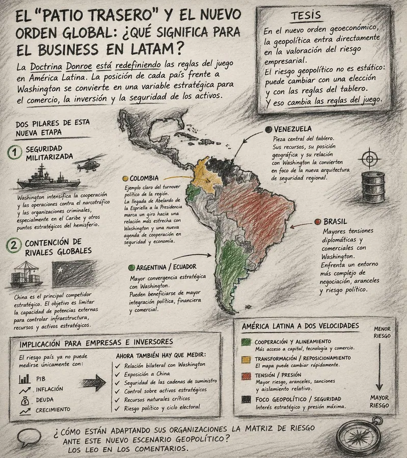
The “Backyard” and the New Global Order: What Does It Mean for the Business Plan in LatAm?
An analysis of how the so-called Donroe Doctrine has turned the “backyard” metaphor into explicit policy, and what that shift means for any business plan built for Latin America.

NOTA-BIO-002 · Bioenergetics
Why do the most efficient workers slow down midway through the workday?
For operations directors and logistics managers: a bioenergetic reading of why top performers lose productivity midway through the workday, a pattern many see and few explain.

NOTA-BIO-003 · Bioenergetics
Threat or opportunity? Artificial intelligence and our creative capacity
Responding to Pope Leo XIV’s call to “disarm AI”, this piece argues that the risk lies not in the technology but in the human system using it: well designed, AI can free up creative capacity.